Drag minimization over an obstacle in Stokes-flow
Section author: Jørgen S. Dokken <dokken@simula.no>
This demo solves the famous shape optimization problem for minimizing drag over an obstacle subject to Stokes flow. This problem was initially analyzed by [1E-Pir74] where the optimal geometry was found to be a rugby shaped ball with a 90 degree front and back wedge.
We start with a circular obstacle in a duct, with an inlet on the left hand side, outlet on the right hand side, and no-slip walls on the top and the bottom.
Shape optimization
We define the change of the fluid domain from its unperturbed state \(\Omega_0\), as \(\Omega(s)=\{x+s(h)\vert x\in \Omega_0 \}\), , and \(s\) is solving a linear elasticity problem [1E-SS16] with a variable Lamé parameter \(\mu\).
where
is the stress and strain tensors, respectively. We set \(\lambda_{elas}=0\), and let \(\mu_{elas}\) solve
As opposed to [1E-SS16], we do not use the the linear elasticity equation as a Riesz-representation of the shape derivative. We instead use the stresses \(h\) in (1) as the design parameters for the problem.
Problem definition
This problem is to find the shape of the obstacle \(\Gamma\), which minimizes the dissipated power in the fluid
where \(\mathrm{Vol}(\Omega)\) is the volume and \(\mathrm{Bc}_j(\Omega)\) is the \(j\)-th component of the barycenter of the obstacle. The state variable \(u\) is a velocity field subject to the Stokes equations:
where \(\Lambda_1\) are the walls, \(\Lambda_2\) the inlet and \(\Lambda_3\) the outlet of the channel.
Implementation
First, the dolfin and dolfin_adjoint modules are imported:
import matplotlib.pyplot as plt
from create_mesh import inflow_marker, outflow_marker, wall_marker, obstacle_marker, c_x, c_y, L, H
from dolfin import *
from dolfin_adjoint import *
set_log_level(LogLevel.ERROR)
Next, we load the facet marker values used in the mesh, as well as some geometrical quantities mesh-generator file.
The initial (unperturbed) mesh and corresponding facet function from their respective xdmf-files.
mesh = Mesh()
with XDMFFile("mesh.xdmf") as infile:
    infile.read(mesh)

mvc = MeshValueCollection("size_t", mesh, 1)
with XDMFFile("mf.xdmf") as infile:
    infile.read(mvc, "name_to_read")
    mf = cpp.mesh.MeshFunctionSizet(mesh, mvc)
We compute the initial volume of the obstacle
one = Constant(1)
Vol0 = L * H - assemble(one * dx(domain=mesh))
We create a Boundary-mesh and function space for our control \(h\)
b_mesh = BoundaryMesh(mesh, "exterior")
S_b = VectorFunctionSpace(b_mesh, "CG", 1)
h = Function(S_b, name="Design")

zero = Constant([0] * mesh.geometric_dimension())
We create a corresponding function space on \(\Omega\), and transfer the corresponding boundary values to the function \(h_V\). This call is needed to be able to represent \(h\) in the variational form of \(s\).
S = VectorFunctionSpace(mesh, "CG", 1)
s = Function(S, name="Mesh perturbation field")
h_V = transfer_from_boundary(h, mesh)
h_V.rename("Volume extension of h", "")
We can now transfer our mesh according to (1).
def mesh_deformation(h):
    # Compute variable :math:`\mu`
    V = FunctionSpace(mesh, "CG", 1)
    u, v = TrialFunction(V), TestFunction(V)

    a = -inner(grad(u), grad(v)) * dx
    l = Constant(0) * v * dx

    mu_min = Constant(1, name="mu_min")
    mu_max = Constant(500, name="mu_max")
    bcs = []
    for marker in [inflow_marker, outflow_marker, wall_marker]:
        bcs.append(DirichletBC(V, mu_min, mf, marker))
    bcs.append(DirichletBC(V, mu_max, mf, obstacle_marker))

    mu = Function(V, name="mesh deformation mu")
    solve(a == l, mu, bcs=bcs)

    # Compute the mesh deformation
    S = VectorFunctionSpace(mesh, "CG", 1)
    u, v = TrialFunction(S), TestFunction(S)
    dObstacle = Measure("ds", subdomain_data=mf, subdomain_id=obstacle_marker)

    def epsilon(u):
        return sym(grad(u))

    def sigma(u, mu=500, lmb=0):
        return 2 * mu * epsilon(u) + lmb * tr(epsilon(u)) * Identity(2)

    a = inner(sigma(u, mu=mu), grad(v)) * dx
    L = inner(h, v) * dObstacle

    bcs = []
    for marker in [inflow_marker, outflow_marker, wall_marker]:
        bcs.append(DirichletBC(S, zero, mf, marker))

    s = Function(S, name="mesh deformation")
    solve(a == L, s, bcs=bcs)
    return s
We compute the mesh deformation with the volume extension of the control variable \(h\) and move the domain.
s = mesh_deformation(h_V)
ALE.move(mesh, s)
The next step is to set up (2). We start by defining the stable Taylor-Hood finite element space.
V2 = VectorElement("CG", mesh.ufl_cell(), 2)
S1 = FiniteElement("CG", mesh.ufl_cell(), 1)
VQ = FunctionSpace(mesh, V2 * S1)
Then, we define the test and trial functions, as well as the variational form
(u, p) = TrialFunctions(VQ)
(v, q) = TestFunctions(VQ)
a = inner(grad(u), grad(v)) * dx - div(u) * q * dx - div(v) * p * dx
l = inner(zero, v) * dx
The Dirichlet boundary conditions on \(\Gamma\) is defined as follows
(x, y) = SpatialCoordinate(mesh)
g = Expression(("sin(pi*x[1])", "0"), degree=2)
bc_inlet = DirichletBC(VQ.sub(0), g, mf, inflow_marker)
bc_obstacle = DirichletBC(VQ.sub(0), zero, mf, obstacle_marker)
bc_walls = DirichletBC(VQ.sub(0), zero, mf, wall_marker)
bcs = [bc_inlet, bc_obstacle, bc_walls]
We solve the mixed equations and split the solution into the velocity-field \(u\) and pressure-field \(p\).
w = Function(VQ, name="Mixed State Solution")
solve(a == l, w, bcs=bcs)
u, p = w.split()
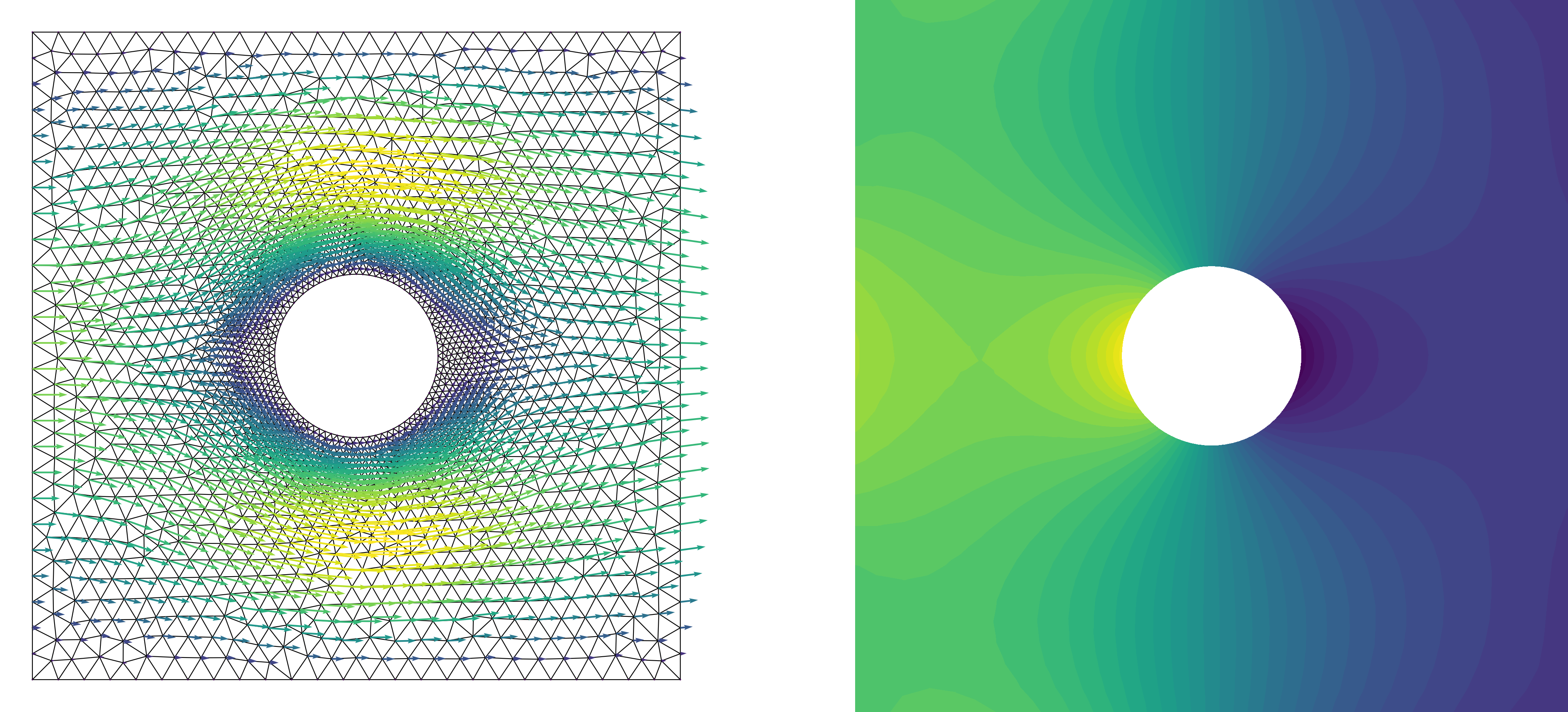
Plotting the initial velocity and pressure
plt.figure()
plt.subplot(1, 2, 1)
plot(mesh, color="k", linewidth=0.2, zorder=0)
plot(u, zorder=1, scale=20)
plt.axis("off")
plt.subplot(1, 2, 2)
plot(p, zorder=1)
plt.axis("off")
plt.savefig("intial.png", dpi=800, bbox_inches="tight", pad_inches=0)
We compute the dissipated energy in the fluid volume, \(\int_{\Omega(s)} \sum_{i,j=1}^2 \left(\frac{\partial u_i}{\partial x_j}\right)^2~\mathrm{d} x\)
J = assemble(inner(grad(u), grad(u)) * dx)
Then, we add a weak enforcement of the volume contraint, \(\alpha\big(\mathrm{Vol}(\Omega(s))-\mathrm{Vol}(\Omega_0)\big)^2\).
alpha = 1e4
Vol = assemble(one * dx(domain=mesh))
J += alpha * ((L * H - Vol) - Vol0)**2
Similarly, we add a weak enforcement of the barycenter contraint, \(\beta\big(\mathrm{Bc}_j(\Omega(s))-\mathrm{Bc}_j(\Omega_0)\big)^2\).
Bc1 = (L**2 * H / 2 - assemble(x * dx(domain=mesh))) / (L * H - Vol)
Bc2 = (L * H**2 / 2 - assemble(y * dx(domain=mesh))) / (L * H - Vol)
beta = 1e4
J += beta * ((Bc1 - c_x)**2 + (Bc2 - c_y)**2)
We define the reduced functional, where \(h\) is the design parameter# and use scipy to minimize the objective.
Jhat = ReducedFunctional(J, Control(h))
s_opt = minimize(Jhat, tol=1e-6, options={"gtol": 1e-6, "maxiter": 50, "disp": True})
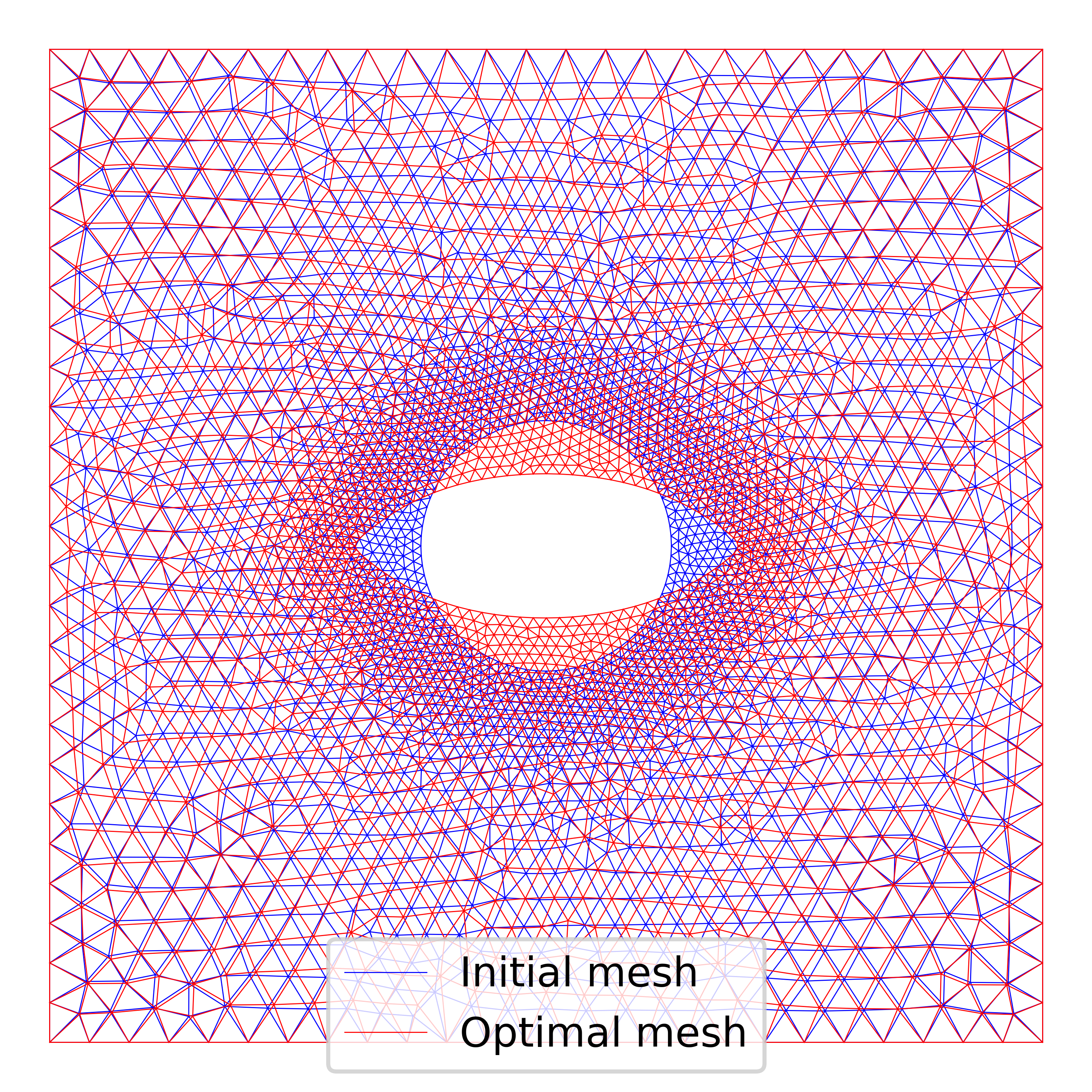
# We evaluate the functional with the optimal solution and plot
# the initial and final mesh
plt.figure()
Jhat(h)
initial, _ = plot(mesh, color="b", linewidth=0.25, label="Initial mesh")
Jhat(s_opt)
optimal, _ = plot(mesh, color="r", linewidth=0.25, label="Optimal mesh")
plt.legend(handles=[initial, optimal])
plt.axis("off")
plt.savefig("meshes.png", dpi=800, bbox_inches="tight", pad_inches=0)
In addition, we perform a Taylor-test to verify the shape gradient and Hessian. We compute the convergence rates and check that they correspond to the expected values.
perturbation = interpolate(Expression(("-A*x[0]", "A*x[1]"),
                                      A=5000, degree=2), S_b)
results = taylor_to_dict(Jhat, Function(S_b), perturbation)
assert(min(results["R0"]["Rate"]) > 0.9)
assert(min(results["R1"]["Rate"]) > 1.95)
assert(min(results["R2"]["Rate"]) > 2.95)
- 1E-Pir74
Olivier Pironneau. On optimum design in fluid mechanics. Journal of Fluid Mechanics, 64(1):97–110, 1974. doi:10.1017/S0022112074002023.
- 1E-SS16(1,2)
Volker Schulz and Martin Siebenborn. Computational comparison of surface metrics for PDE constrained shape optimization. Computational Methods in Applied Mathematics, 16(3):485–496, 2016. doi:10.1515/cmam-2016-0009.