
Learning Reaction Rates of an Advection-Diffusion-Reaction System
Section author: Marius Causemann <mariusca@simula.no>
In this demo we try to learn the chemical reaction rates of an advection-diffusion-reaction system from data. It is based on the advection-diffusion-reaction example in the FEniCS tutorial and uses a feed-forward neural network defined in the UFL language to model the reaction rate. Instead of relying on UFL, it also possible to couple dolfin-adjoint with a machine learning framework such as Pytorch for more complex architectures (see e.g. [Bar18], https://github.com/barkm/grey-box).

The system consists of three different chemical species A, B and C, that are advected by an underlying velocity field \(w\), diffuse through the domain \(\Omega\) with diffusivity \(\epsilon\) and obey the following reaction scheme:
With the unknown reaction rate:
We denote the concentrations of A, B and C with \(u_1\), \(u_2\) and \(u_3\) and add source terms \(f_1\), \(f_2\) and \(f_3\) for each species, respectively. Then the coupled system of nonlinear PDEs reads:
Now, we model the unkown reaction rate \(R\) with a neural network (NN) \(R_{\theta}(u_1, u_2)\) parameterized with the weights \(\theta\) and formulate the resulting hybrid PDE-NN problem as a PDE-constrained optimization problem as introduced in [MFK21].
Problem Definition
Assuming that we can observe the concentrations \(u_i^{\star}\) of all species i at all points in time in the whole domain, we set the goal to minimize the weighted \(L^2\) error:
subject to:
with initial conditions \(u_{i}=0\) for \(i=1,2,3\). The weights \(\lambda_i\) of the minimization functional are introduced to account for the smaller magnitude of the concentration of the newly formed species C.
FEniCS implementation
For the details of the implementation of the background velocity field and the advection-diffusion-reaction system, we refer to the FEniCS tutorial. Here, we implement a function solve_reaction_system that solves the reaction system for a given reaction funtion (reaction_func) and computes the loss for each time step, if a loss function (loss_func) is provided:
from fenics import *
from fenics_adjoint import *
set_log_level(LogLevel.CRITICAL)

def solve_reaction_system(mesh, T, num_steps, reaction_func, loss_func=lambda n,x: 0):

    dt = T / num_steps # time step size
    eps = 0.01         # diffusion coefficient

    # Define function space for velocity
    W = VectorFunctionSpace(mesh, 'CG', 2)

    # Define function space for system of concentrations
    P1 = FiniteElement('CG', triangle, 1)
    element = MixedElement([P1, P1, P1])
    V = FunctionSpace(mesh, element)

    # Define test functions
    v_1, v_2, v_3 = TestFunctions(V)

    # Define functions for velocity and concentrations
    w = Function(W)
    u = Function(V)
    u_n = Function(V)

    # Split system functions to access components
    u_1, u_2, u_3 = split(u)
    u_n1, u_n2, u_n3 = split(u_n)

    # Define source terms
    f_1 = Expression('pow(x[0]-0.1,2)+pow(x[1]-0.1,2)<0.05*0.05 ? 10 : 0',
                     degree=1)
    f_2 = Expression('pow(x[0]-0.1,2)+pow(x[1]-0.3,2)<0.05*0.05 ? 10 : 0',
                     degree=1)
    f_3 = Constant(0)

    # Define expressions used in variational forms
    k = Constant(dt)
    eps = Constant(eps)

    # Define variational problem
    F = (((u_1 - u_n1) / k)*v_1*dx + dot(w, grad(u_1))*v_1*dx
      + eps*dot(grad(u_1), grad(v_1))*dx + reaction_func(u_1, u_2)*v_1*dx
      + ((u_2 - u_n2) / k)*v_2*dx + dot(w, grad(u_2))*v_2*dx
      + eps*dot(grad(u_2), grad(v_2))*dx + reaction_func(u_1, u_2)*v_2*dx
      + ((u_3 - u_n3) / k)*v_3*dx + dot(w, grad(u_3))*v_3*dx
      + eps*dot(grad(u_3), grad(v_3))*dx - reaction_func(u_1, u_2)*v_3*dx
      - f_1*v_1*dx - f_2*v_2*dx - f_3*v_3*dx)

    inflow   = 'near(x[0], 0)'
    bc_inflow = DirichletBC(V, Constant((0,0,0)), inflow)

    # Create time series for reading velocity data
    timeseries_w = TimeSeries('navier_stokes_cylinder/velocity_series')
    timeseries_w.retrieve(w.vector(), 2.0)

    # Time-stepping
    t = 0
    results = []
    loss = 0.0
    for n in range(num_steps):

        # Update current time
        t += dt

        # Solve variational problem for time step
        solve(F == 0, u, bcs=bc_inflow)

        # Save solution to file (VTK)
        _u_1, _u_2, _u_3 = u.split()
        _u_1.rename("u1","u1")
        _u_2.rename("u2","u3")
        _u_3.rename("u3","u3")

        # Update previous solution
        u_n.assign(u)
        loss += loss_func(n, u.split())
        results.append(u.copy())

    return loss, results
For the NN part, we rely on the NN implementation by [MFK21].
Putting those two components together, we can define the hybrid PDE-NN training problem in a few lines of code. First, we generate the ground truth training data with the reaction rate \(R(u_1, u_2)= K u_1 u_2\):
from neural_network import ANN
import numpy as np
import matplotlib.pyplot as plt

np.random.seed(99)

T = 2.0
num_steps = 20
K = Constant(10)

mesh = Mesh('navier_stokes_cylinder/cylinder.xml.gz')

#ground truth reaction term
def R_true(u1, u2):
        return K*u1*u2

#create ground_truth data
_, ground_truth = solve_reaction_system(mesh, T, num_steps, R_true)
Next, we define a neural network with one hidden layer with 10 neurons, two scalar input values and a single scalar output:
layers = [2, 10, 1]
bias = [True , True]
net = ANN(layers, bias=bias, mesh=mesh)

def R_net(u1, u2):
    return net([u1, u2])
Now, we specify the loss function and compute the loss with the initial weights of the NN:
#define L2 loss function for each timestep i.
#As the concentrations of u_3 are much smaller, we put more weight on it.
loss_weights = [1,1, 200]

def loss_func(n, data):
    loss = 0.0
    for u in [0,1,2]:
        loss += loss_weights[u]*assemble((data[u] - ground_truth[n][u])**2*dx)
    return loss

# solve reaction system and compute loss with initial weights
loss, learned_data = solve_reaction_system(mesh,T, num_steps, R_net,
                                           loss_func=loss_func)
Then, we start the training process using the scipy L-BFGS-optimizer for 100 iterations. Note that the training process can take a significant amout of time, since at least one solve of the forward and adjoint equation is required per training iteration.
#define reduced functional
J_hat = ReducedFunctional(loss, net.weights_ctrls())

#Use scipy L - BFGS optimiser
opt_weights = minimize(J_hat, method ="L-BFGS-B", tol = 1e-6,
                       options = {'disp': True, "maxiter":100})
net.set_weights(opt_weights)
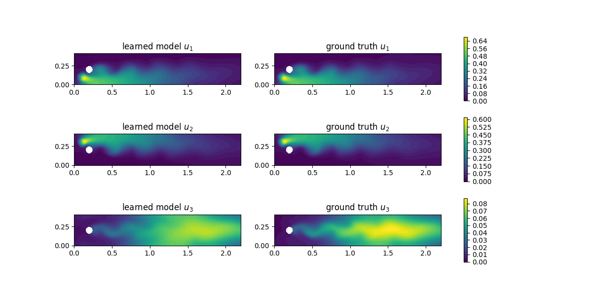
For evaluation, we compute the concentrations with the learned reaction rates at final time and observe a good agreement:
# compute final learned state
final_loss, learned_data = solve_reaction_system(mesh,T, num_steps, R_net,
                                                 loss_func=loss_func)

# plot concentrations at final time
i = num_steps - 1
fig, axs = plt.subplots(nrows=3, ncols=2, figsize=(12,6))

for u in [0,1,2]:
    u_max = ground_truth[i].split(deepcopy=True)[u].vector()[:].max()
    plt.axes(axs[u,0])
    plt.title(f"learned model $u_{u+1}$")
    plot(learned_data[i][u], vmin=0, vmax=u_max)
    plt.axes(axs[u,1])
    plt.title(f"ground truth $u_{u+1}$")
    im = plot(ground_truth[i][u], vmin=0, vmax=u_max)
    cbar = fig.colorbar(im, ax=axs[u,:], shrink=0.95)

plt.savefig("concentrations.png")
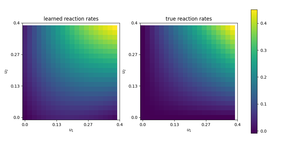
Finally, we are also interested in the learned reaction rates:
# plot learned reaction rates
n = 20
c_max = 0.4
n_ticks = 4
ticks = np.round(np.linspace(0,c_max, n_ticks),2)
learned_rates = np.zeros(shape=(n,n))
exact_rates = np.zeros(shape=(n,n))
concentrations = np.linspace(0,c_max, n)

for i,c1 in enumerate(concentrations):
    for j,c2 in enumerate(concentrations):
        learned_rates[i,j] = net([Constant(c1), Constant(c2)])([0.0,0.0])
        exact_rates[i,j] = c1*c2*K.values()[0]

vmax = max([learned_rates.max()])#, exact_rates.max()])
fig, axs = plt.subplots(1,2, figsize = (10,5))
plt.axes(axs[0])
plt.title("learned reaction rates")
im = plt.imshow(learned_rates, origin="lower",vmax=vmax)
plt.xticks( np.linspace(0,n, n_ticks), ticks)
plt.yticks( np.linspace(0,n, n_ticks), ticks)
plt.xlabel("$u_1$")
plt.ylabel("$u_2$")

plt.axes(axs[1])
plt.title("true reaction rates")
plt.imshow(exact_rates, origin="lower")
plt.xticks( np.linspace(0,n, n_ticks), ticks)
plt.yticks( np.linspace(0,n, n_ticks), ticks)
plt.xlabel("$u_1$")
plt.ylabel("$u_2$")

plt.tight_layout()
cbar = fig.colorbar(im, ax=axs, shrink=0.95)

plt.savefig("learned_reaction_rates.png")
- Bar18
Patrik Barkman. Grey-box modelling of distributed parameter systems. Master's thesis, KTH, School of Electrical Engineering and Computer Science (EECS), 2018.
- MFK21(1,2)
Sebastian K Mitusch, Simon W Funke, and Miroslav Kuchta. Hybrid fem-nn models: combining artificial neural networks with the finite element method. arXiv preprint arXiv:2101.00962, 2021.