Debugging
Visualising the system
It is sometimes useful when debugging a problem to see dolfin-adjoint’s
interpretation of your forward system, and the other models it derives
from that. The visualise function
visualises the system as a graph using TensorFlow. To do this add
tape = get_working_tape()
tape.visualise()
This will create a log directory with TensorFlow event files. We can then run TensorBoard, which comes bundled with TensorFlow, and point it to this log directory:
tensorboard --logdir=log
By default the log directory is a directory log in the
current working directory. This can be changed by specifying a
directory in the logdir keyword argument to
visualise.
Finally, we can open http://localhost:6006/ in a web browser to view the graph. To demonstrate, let us use a simplified version of our old Burgers’ equation example:
from dolfin import *
from fenics_adjoint import *

n = 30
mesh = UnitSquareMesh(n, n)
V = VectorFunctionSpace(mesh, "CG", 2)

u = project(Expression(("sin(2*pi*x[0])", "cos(2*pi*x[1])"), degree=2),  V)
u_next = Function(V)
v = TestFunction(V)

nu = Constant(0.0001)

timestep = Constant(0.01)

F = (inner((u_next - u)/timestep, v)
     + inner(grad(u_next)*u_next, v)
     + nu*inner(grad(u_next), grad(v)))*dx

bc = DirichletBC(V, (0.0, 0.0), "on_boundary")

solve(F == 0, u_next, bc)

tape = get_working_tape()
tape.visualise()
Here we solve the equation for only one timestep.
 Download the code to find graph.
Running TensorBoard and opening http://localhost:6006/ in our web browser shows us the following graph:
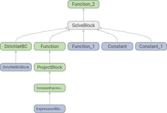
Each node corresponds to an elementary operation, and we see that the structure is what we should expect: two functions, two constants and a set of boundary conditions go into an equation and we get one function out. To increase readability further we can add names to the functions:
from dolfin import *
from fenics_adjoint import *

n = 30
mesh = UnitSquareMesh(n, n)
V = VectorFunctionSpace(mesh, "CG", 2)

u = project(Expression(("sin(2*pi*x[0])", "cos(2*pi*x[1])"), degree=2),  V)
u_next = Function(V, name="u_next")
v = TestFunction(V)

nu = Constant(0.0001, name="nu")

timestep = Constant(0.01, name="dt")

F = (inner((u_next - u)/timestep, v)
     + inner(grad(u_next)*u_next, v)
     + nu*inner(grad(u_next), grad(v)))*dx

bc = DirichletBC(V, (0.0, 0.0), "on_boundary")

solve(F == 0, u_next, bc)

tape = get_working_tape()
tape.visualise()
The resulting graph is the following:
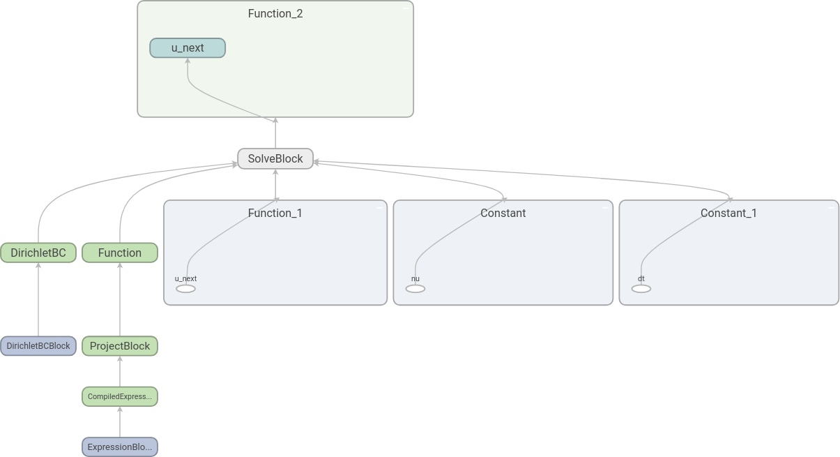
Here we have expanded some of the nodes by double-clicking on them. We
see that it is indeed u_next that is found by the equation
solve.
Download the code to find the graph with names.
If we have a time loop, the graph can easily become large and difficult
to read. The name_scope factory
function can be used to make this easier. To demonstrate this, we add a
time loop to our example above:
from dolfin import *
from fenics_adjoint import *

n = 30
mesh = UnitSquareMesh(n, n)
V = VectorFunctionSpace(mesh, "CG", 2)

u = project(Expression(("sin(2*pi*x[0])", "cos(2*pi*x[1])"), degree=2),  V)
u_next = Function(V, name="u_next")
v = TestFunction(V)

nu = Constant(0.0001, name="nu")

timestep = Constant(0.01, name="dt")

F = (inner((u_next - u)/timestep, v)
     + inner(grad(u_next)*u_next, v)
     + nu*inner(grad(u_next), grad(v)))*dx

bc = DirichletBC(V, (0.0, 0.0), "on_boundary")

tape = get_working_tape()

t = 0.0
end = 0.05
while (t <= end):
    with tape.name_scope("Timestep"):
        solve(F == 0, u_next, bc)
        u.assign(u_next)
        t += float(timestep)

tape.visualise()
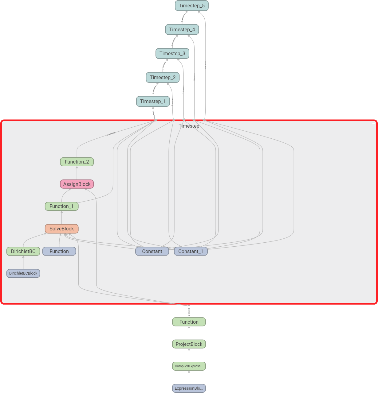
Here, we should note the line after we enter the while
loop. In this line we use a with statement together with
name_scope and a name for the
scope. This will ensure that all nodes corresponding to one time step
will be added to its own scope. After the time loop, we call
visualise and get the following
graph:
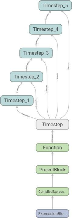
We can then expand the scopes as we like. Here we have expanded the first time step:
Download the code to find the graph with name scopes.
In the next section we discuss parallelisation.