Dirichlet BC control of the Stokes equations
Section author: Simon W. Funke <simon@simula.no>, André Massing <massing@simula.no>
This example demonstrates how to compute the sensitivity with respect to the Dirichlet boundary conditions in pyadjoint.
Problem definition
Consider the problem of minimising the compliance
subject to the Stokes equations
with Dirichlet boundary conditions
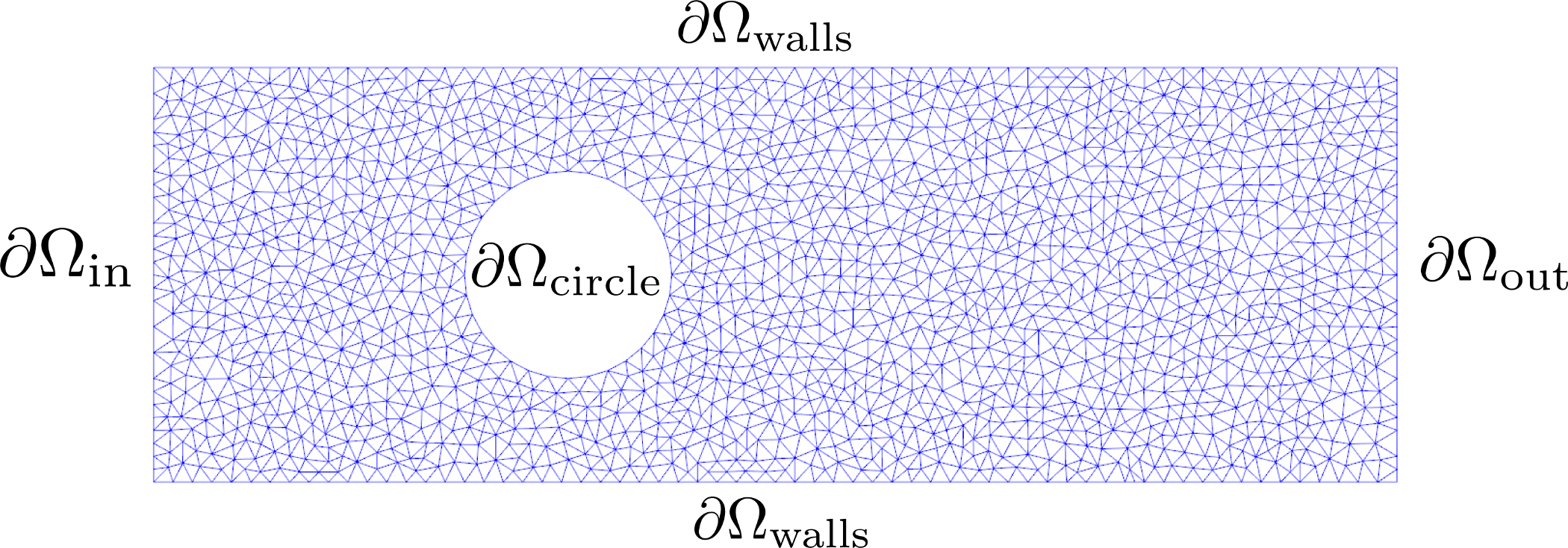
where \(\Omega\) is the domain of interest (visualised below), \(u:\Omega \to \mathbb R^2\) is the unknown velocity, \(p:\Omega \to \mathbb R\) is the unknown pressure, \(\nu\) is the viscosity, \(\alpha\) is the regularisation parameter, \(f\) denotes the value for the Dirichlet inflow boundary condition, and \(g\) is the control variable that specifies the Dirichlet boundary condition on the circle.
Physically, this setup corresponds to minimising the loss of flow energy into heat by actively controlling the in/outflow at the circle boundary. To avoid excessive control solutions, non-zero control values are penalised via the regularisation term.
Implementation
First, the dolfin and dolfin_adjoint modules are imported:
from dolfin import *
from dolfin_adjoint import *
set_log_level(LogLevel.ERROR)
Next, we load the mesh. The mesh was generated with mshr; see make-mesh.py in the same directory.
mesh_xdmf = XDMFFile(MPI.comm_world, "rectangle-less-circle.xdmf")
mesh = Mesh()
mesh_xdmf.read(mesh)
Then, we define the discrete function spaces. A Taylor-Hood finite-element pair is a suitable choice for the Stokes equations. The control function is the Dirichlet boundary value on the velocity field and is hence be a function on the velocity space (note: FEniCS cannot restrict functions to boundaries, hence the control is defined over the entire domain).
V_h = VectorElement("CG", mesh.ufl_cell(), 2)
Q_h = FiniteElement("CG", mesh.ufl_cell(), 1)
W = FunctionSpace(mesh, V_h * Q_h)
V, Q = W.split()

v, q = TestFunctions(W)
x = TrialFunction(W)
u, p = split(x)
s = Function(W, name="State")
V_collapse = V.collapse()
g = Function(V_collapse, name="Control")

nu = Constant(1)
Our functional requires the computation of a boundary integral
over \(\partial \Omega_{\textrm{circle}}\). Therefore, we need
to create a measure for this integral, which will be accessible as
ds(2) in the definition of the functional. In addition, we
define our strong Dirichlet boundary conditions.
# Define the circle boundary
class Circle(SubDomain):
    def inside(self, x, on_boundary):
        return on_boundary and (x[0]-10)**2 + (x[1]-5)**2 < 3**2

facet_marker = MeshFunction("size_t", mesh, mesh.topology().dim() - 1)
facet_marker.set_all(10)
Circle().mark(facet_marker, 2)

# Define a boundary measure with circle boundary tagged.
ds = ds(subdomain_data=facet_marker)

# Define boundary conditions
u_inflow = Expression(("x[1]*(10-x[1])/25", "0"), degree=1)
noslip = DirichletBC(W.sub(0), (0, 0),
                     "on_boundary && (x[1] >= 9.9 || x[1] < 0.1)")
inflow = DirichletBC(W.sub(0), u_inflow, "on_boundary && x[0] <= 0.1")
circle = DirichletBC(W.sub(0), g, facet_marker, 2)
bcs = [inflow, noslip, circle]
We derive the standard weak formulation of the Stokes problem: Find \(u, p\) such that for all test functions \(v, q\)
with
In code, this becomes:
a = (nu*inner(grad(u), grad(v))*dx
     - inner(p, div(v))*dx
     - inner(q, div(u))*dx
     )
L = inner(Constant((0, 0)), v)*dx
Next we assemble and solve the system once to record it with
dolin-adjoint.
A, b = assemble_system(a, L, bcs)
solve(A, s.vector(), b)
Next we define the functional of interest \(J\), the optimisation parameter \(g\), and create the reduced functional.
u, p = split(s)
alpha = Constant(10)

J = assemble(1./2*inner(grad(u), grad(u))*dx + alpha/2*inner(g, g)*ds(2))
m = Control(g)
Jhat = ReducedFunctional(J, m)
Now, everything is set up to run the optimisation and to plot the
results. By default, minimize() uses the L-BFGS-B
algorithm.
g_opt = minimize(Jhat, options={"disp": True})
plot(g_opt, title="Optimised boundary")

g.assign(g_opt)
A, b = assemble_system(a, L, bcs)
solve(A, s.vector(), b)
plot(s.sub(0), title="Velocity")
plot(s.sub(1), title="Pressure")
Results
The example code can be found in examples/stokes-bc-control in
the dolfin-adjoint source tree, and executed as follows:
$ python stokes-bc-control.py
  ...
  At iterate   19    f=  1.99805D+01    |proj g|=  3.73343D-04

  At iterate   20    f=  1.99805D+01    |proj g|=  1.34691D-04

  At iterate   21    f=  1.99805D+01    |proj g|=  6.16572D-05

             * * *

  Tit   = total number of iterations
  Tnf   = total number of function evaluations
  Tnint = total number of segments explored during Cauchy searches
  Skip  = number of BFGS updates skipped
  Nact  = number of active bounds at final generalized Cauchy point
  Projg = norm of the final projected gradient
  F     = final function value

             * * *

     N    Tit     Tnf  Tnint  Skip  Nact     Projg        F
  15708     21     26      1     0     0   6.166D-05   1.998D+01
    F =   19.980459647407621

  CONVERGENCE: REL_REDUCTION_OF_F_<=_FACTR*EPSMCH

   Cauchy                time 0.000E+00 seconds.
   Subspace minimization time 0.000E+00 seconds.
   Line search           time 0.000E+00 seconds.

   Total User time 0.000E+00 seconds.
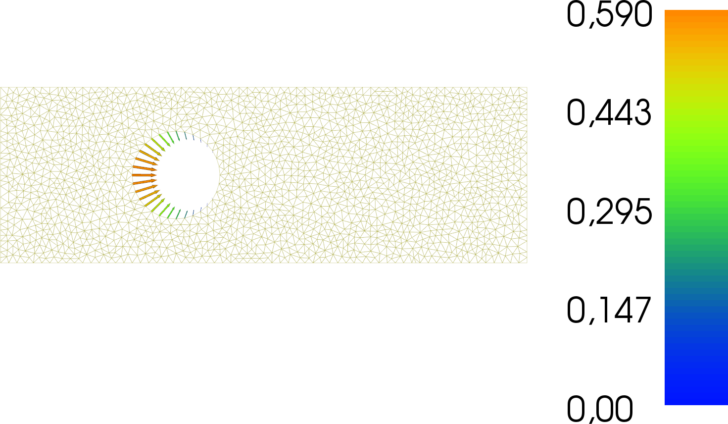
The results are visualised in the following images. The first image shows the optimised control function, i.e. the Dirichlet values on the circle boundary which minimise the loss of flow energy into heat.
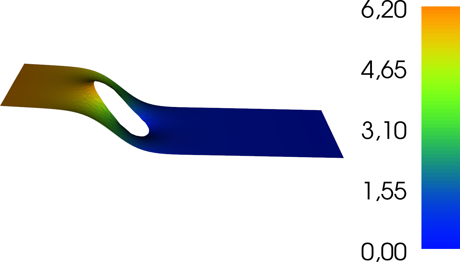
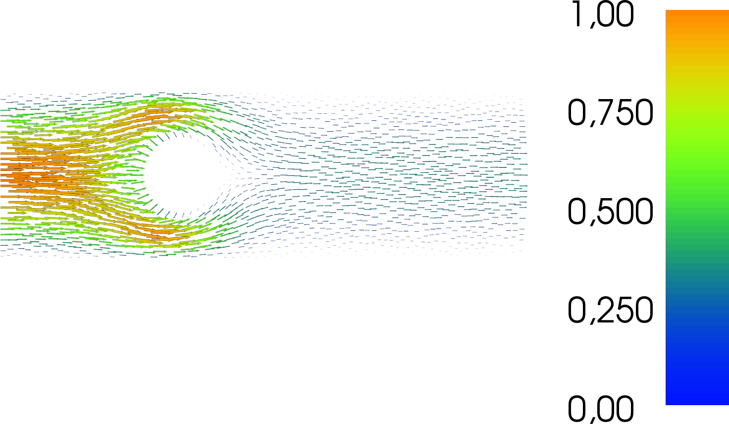
The next image shows the associated velocity:
And the final image shows the pressure: