
Optimal control of the Poisson equation
Section author: Simon W. Funke <simon@simula.no>
This demo solves the mother problem of PDE-constrained optimisation: the optimal control of the Poisson equation. Physically, this problem can the interpreted as finding the best heating/cooling of a cooktop to achieve a desired temperature profile.
This example introduces the basics of how to solve optimisation problems with dolfin-adjoint.
Problem definition
Mathematically, the problem is to minimise the following tracking-type functional
subject to the Poisson equation with Dirichlet boundary conditions
where \(\Omega\) is the domain of interest (here the unit square), \(u: \Omega \to \mathbb R\) is the unkown temperature, \(\kappa \in \mathbb R\) is the thermal diffusivity (here: \(\kappa = 1\)), \(f: \Omega \to \mathbb R\) is the unknown control function acting as source term (\(f(x) > 0\) corresponds to heating and \(f(x) < 0\) corresponds to cooling), \(d: \Omega \to \mathbb R\) is the given desired temperature profile, \(\alpha \in [0, \infty)\) is a Tikhonov regularisation parameter, and \(a, b: \Omega \to \mathbb R\) are lower and upper bounds for the control function.
It can be shown that this problem is well-posed and has a unique solution, see [1E-Troltzsch10] or section 1.5 of [1M-HPUU09].
Implementation
We start our implementation by importing the dolfin and
dolfin_adjoint modules:
from dolfin import *

from dolfin_adjoint import *
Next we import the Python interface to Moola. Moola is a collection of optimisation solvers specifically designed for PDE-constrained optimisation problems. If Moola is not yet available on your system, it is easy to install.
import moola
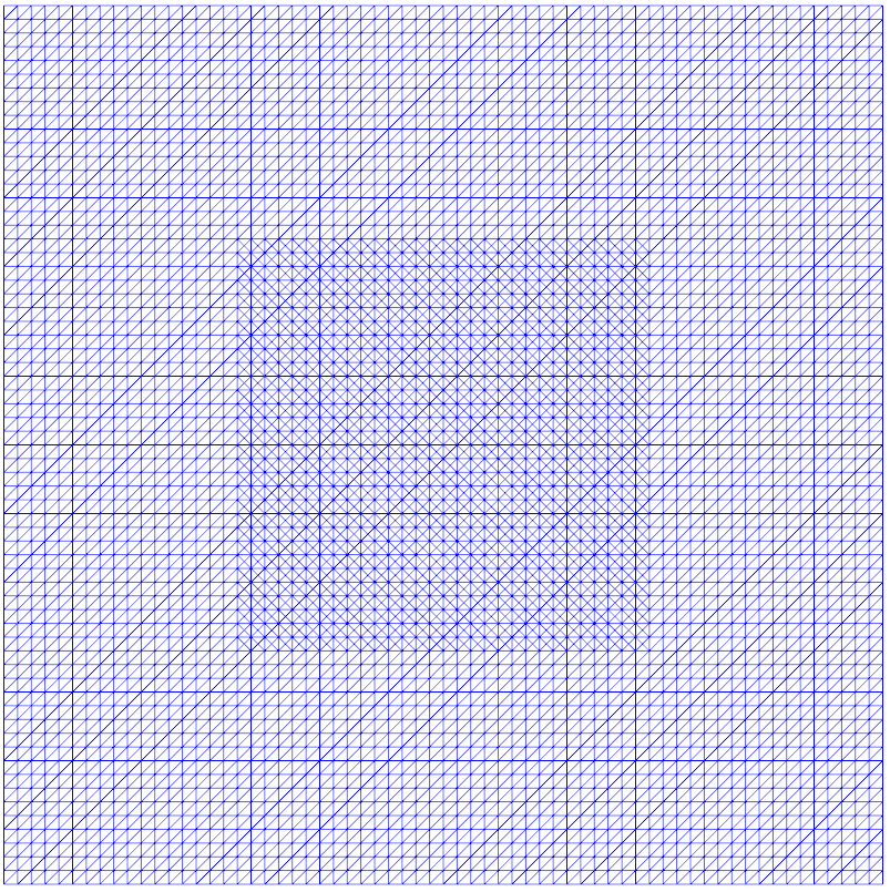
Next we create a regular mesh of the unit square. Some optimisation algorithms suffer from bad performance when the mesh is non-uniform (i.e. when the mesh is partially refined). To demonstrate that Moola does not have this issue, we refine the mesh near the center of the domain:
n = 64
mesh = UnitSquareMesh(n, n)

cf = MeshFunction("bool", mesh, mesh.geometric_dimension())
subdomain = CompiledSubDomain('std::abs(x[0]-0.5) < 0.25 && std::abs(x[1]-0.5) < 0.25')
subdomain.mark(cf, True)
mesh = refine(mesh, cf)
The resulting mesh looks like this:
Then we define the discrete function spaces and create functions for the temperature and the control function.
V = FunctionSpace(mesh, "CG", 1)
W = FunctionSpace(mesh, "DG", 0)

f = interpolate(Expression("x[0]+x[1]", name='Control', degree=1), W)
u = Function(V, name='State')
v = TestFunction(V)
The optimisation algorithm will use the value of the control function \(f\) as an initial guess for the optimisation. A zero-initial guess for the control appears to be too simple: for example L-BFGS finds the optimal control with just two iterations. To make it more interesting, we chose a non-zero initial guess instead.
Next we define the weak formulation of the Poisson problem and solve it.
F = (inner(grad(u), grad(v)) - f * v) * dx
bc = DirichletBC(V, 0.0, "on_boundary")
solve(F == 0, u, bc)
By doing so, dolfin-adjoint automatically records the details of each PDE solve (also called a tape). This tape will be used by the optimisation algorithm to repeatedly solve the forward and adjoint problems for varying control inputs.
Before we can start the optimisation, we need to specify the control variable and define the functional of interest. For this example we use \(d(x, y) = \frac{1}{2\pi^2}\sin(\pi x)\sin(\pi y)\) as the desired temperature profile, and choose \(f\) as the control variable.
x = SpatialCoordinate(mesh)
w = Expression("sin(pi*x[0])*sin(pi*x[1])", degree=3)
d = 1 / (2 * pi ** 2)
d = Expression("d*w", d=d, w=w, degree=3)

alpha = Constant(1e-6)
J = assemble((0.5 * inner(u - d, u - d)) * dx + alpha / 2 * f ** 2 * dx)
control = Control(f)
The next step is to formulate the so-called reduced optimisation problem. The idea is that the solution \(u\) can be considered as a function of \(f\): given a value for \(f\), we can solve the Poisson equation to obtain the associated solution \(u\). By denoting this solution function as \(u(f)\), we can write the original optimisation problem as a reduced problem:
Note that no PDE-constraint is required anymore, since it is implicitly contained in the solution function.
dolfin-adjoint can automatically reduce the optimisation problem
by creating a ReducedFunctional object. This object
solves the forward PDE using dolfin-adjoint’s tape each time the
functional is to be evaluated, and derives and solves the adjoint
equation each time the functional gradient is to be evaluated.
rf = ReducedFunctional(J, control)
Now that all the ingredients are in place, we can perform the optimisation.
Next we use MoolaOptimizationProblem to generate a problem that
is compatible with the Moola optimisation framework. Then, we
wrap the control function into a Moola object, and create a
NewtonCG() solver for solving the optimisation problem:
problem = MoolaOptimizationProblem(rf)
f_moola = moola.DolfinPrimalVector(f)
solver = moola.NewtonCG(problem, f_moola, options={'gtol': 1e-9,
                                                   'maxiter': 20,
                                                   'display': 3,
                                                   'ncg_hesstol': 0})
Alternatively an L-BFGS solver could initialised by:
solver = moola.BFGS(problem, f_moola, options={'jtol': 0,
                                               'gtol': 1e-9,
                                               'Hinit': "default",
                                               'maxiter': 100,
                                               'mem_lim': 10})
Then we can solve the optimisation problem, extract the optimal control and plot it:
sol = solver.solve()
f_opt = sol['control'].data

plot(f_opt, title="f_opt")

# Define the expressions of the analytical solution
f_analytic = Expression("1/(1+alpha*4*pow(pi, 4))*w", w=w, alpha=alpha, degree=3)
u_analytic = Expression("1/(2*pow(pi, 2))*f", f=f_analytic, degree=3)
We can then compute the errors between numerical and analytical solutions.
f.assign(f_opt)
solve(F == 0, u, bc)
control_error = errornorm(f_analytic, f_opt)
state_error = errornorm(u_analytic, u)
print("h(min):           %e." % mesh.hmin())
print("Error in state:   %e." % state_error)
print("Error in control: %e." % control_error)
The example code can be found in examples/poisson-mother in the
dolfin-adjoint source tree, and executed as follows:
$ python poisson-mother.py
...
Convergence order and mesh independence
It is highly desirable that the optimisation algorithm achieve mesh independence: i.e., that the required number of optimisation iterations is independent of the mesh resolution. Achieving mesh independence requires paying careful attention to the inner product structure of the function space in which the solution is sought.
For our desired temperature, the analytical solutions of the optimisation problem is:
The following numerical experiments solve the optimisation problem for a sequence of meshes with increasing resolutions and record the numerical error and the required number of optimisation iterations. A regularisation coefficient of \(\alpha = 10^{-6}\) was used, and the optimisation was stopped when the \(L_2\) norm of the reduced functional gradient dropped below \(10^{-9}\).
Moola Newton-CG
The Moola Newton-CG algorithm implements an inexact Newton method. Hence, even though the optimality system of our problem is linear, we can not expect the algorithm to converge in a single iteration (however, we could it enforce that by explicitly setting the relative tolerance of the CG algorithm to zero).
Running the Newton-CG algorithm for the different meshes yielded:
| Mesh element size | Newton iterations | CG iterations | Error in control |
|---|---|---|---|
| 6.250e-02 | 3 | 54 | 3.83e-02 |
| 3.125e-02 | 3 | 59 | 1.69e-02 |
| 1.563e-02 | 3 | 57 | 8.05e-03 |
| 7.813e-03 | 3 | 58 | 3.97e-03 |
Here CG iterations denotes the total number of CG iterations during the optimisation. Mesh independent convergence can be observed, both in the Newton and CG iterations.
From our choice of discretisation (\(DG_0\) for \(f\)), we expect a 1st order of convergence for the control variable. Indeed, the error column in the numerical experiments confirm that this rate is obtained in practice.
Moola L-BFGS
The L-BFGS algorithm in Moola implements the limited memory quasi Newton method with Broyden-Fletcher-Goldfarb-Shanno updates. For the numerical experiments, the set of the memory history was set to 10.
The numerical results yield:
| Mesh element size | L-BFGS iterations | Error in control |
|---|---|---|
| 6.250e-02 | 53 | 3.83e-02 |
| 3.125e-02 | 50 | 1.69e-02 |
| 1.563e-02 | 57 | 8.05e-03 |
| 7.813e-03 | 56 | 3.97e-03 |
Again a mesh-independent convergence and a 1st order convergence of the control can be observed.
| [1M-HPUU09] | M. Hinze, R. Pinnau, M. Ulbrich, and S. Ulbrich. Optimization with PDE constraints. Volume 23 of Mathematical Modelling: Theory and Applications. Springer, 2009. ISBN 978-1-4020-8838-4. |
| [1E-Troltzsch10] | F. Tröltzsch. Optimal control of partial differential equations: Theory, methods and applications. Volume 112 of Graduate Studies in Mathematics. AMS, 2010. ISBN 978-0821849040. |