
Mathematical Programs with Equilibrium Constraints
Section author: Simon W. Funke <simon@simula.no>
This demo solves example 5.2 of [5E-HintermullerK11].
Problem definition
This problem is to minimise
subject to the variational inequality
and control constraints
where \(u\) is the control, \(y\) is the solution of the variational inequality, \(y_d\) is data to be matched, \(f\) is a prescribed source term, \(\nu\) is a regularisation parameter and \(a, b\) are upper and lower bounds for the control.
This problem is fundamentally different to a PDE-constrained optimisation problem in that the constraint is not a PDE, but a variational inequality. Such problems are called Mathematical Programs with Equilibrium Constraints (MPECs) and have applications in engineering design (e.g. to determine optimal trajectories for robots [5E-YG05] or process optimisation in chemical engineering [5E-BRB08]) and in economics (e.g. in leader-follower games [5E-LM05] and optimal pricing [5E-LH04]).
Even though it is known that the above problem admits a unique solution, there are some difficulties to be considered when solving MPECs:
- the set of feasible points is in general not necessarly convex or connected, and
- the reduced problem is not Fréchet-differentiable.
Following [5E-HintermullerK11], we will overcome these issues in the next section with a penalisation approach. For a more thorough discussion on MPECs, see [5E-ZQJSD96] and the references therein.
Penalisation technique
A common approach for solving variational inequalities is to
approximate them by a sequence of nonlinear PDEs with a penalisation
term. We transform the above problem into a sequence of
PDE-constrained optimisation problems, which can be solved with
dolfin-adjoint.
For the above problem we use the approximation
where \(\alpha > 0\) is the penalty parameter and the penalty term is defined as
This approximation yields solutions which converge to the solution of the variational inequality as \(\alpha \to 0\) (see chapter IV of [5E-KS00]).
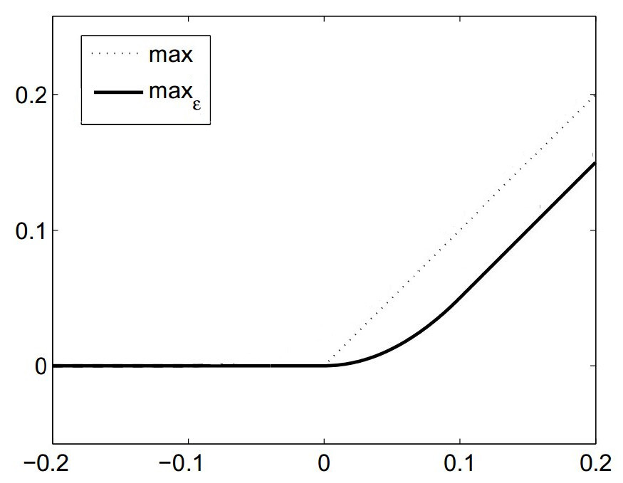
In order to be able to apply a gradient-based optimisation method, we need differentiabilty of the above equation. The \(\max\) operator is not differentiable at the origin, and hence it is replaced by a smooth (\(C^1\)) approximation (plot modified from [5E-HintermullerK11]):
The domain for the example problem is the unit square \(\Omega = (0, 1)^2\). The data and the source term are given as \(y_d(x, y) = f(x, y) = -|xy - 0.5| + 0.25\). The remaining parameters are \(a = 0.01\), \(b = 0.03\) and \(\nu = 0.01\).
Implementation
First, the dolfin and dolfin_adjoint modules are
imported. We also tell DOLFIN to only print error messages to keep the
output comprehensible:
from dolfin import *
from ufl.operators import Max

from dolfin_adjoint import *
from pyadjoint.placeholder import Placeholder

set_log_level(LogLevel.ERROR)

# Needed to have a nested conditional
parameters["form_compiler"]["representation"] = "uflacs"
Next, we define the smooth approximation \(\max_{\epsilon}\) of the maximum operator:
def smoothmax(r, eps=1e-4):
    return conditional(gt(r, eps), r - eps / 2, conditional(lt(r, 0), 0, r ** 2 / (2 * eps)))
Now, we are ready to mesh the domain and define the discrete function spaces. For this example we use piecewise linear, continuous finite elements for both the solution and control.
mesh = UnitSquareMesh(128, 128)
V = FunctionSpace(mesh, "CG", 1)  # The function space for the solution and control functions
y = Function(V, name="Solution")
# Define a Control for the initial guess so we can modify it later.
ic = Control(y)
u = Function(V, name="Control")
w = TestFunction(V)
Next, we define and solve the variational formulation of the PDE
constraint with the penalisation parameter set to
\(\alpha=10^{-2}\). This initial value of \(\alpha\) will
then be iteratively reduced to better approximate the underlying MPEC.
To ensure that new values of \(\alpha\) are reflected on the tape,
we define a Placeholder before using it.
alpha = Constant(1e-2)
Placeholder(alpha)
# The source term
f = interpolate(Expression("-std::abs(x[0]*x[1] - 0.5) + 0.25", degree=1), V)
F = inner(grad(y), grad(w)) * dx - 1 / alpha * inner(smoothmax(-y), w) * dx - inner(f + u, w) * dx
bc = DirichletBC(V, 0.0, "on_boundary")
solve(F == 0, y, bcs=bc)
With the forward problem solved once, dolfin_adjoint has
built a tape of the forward model; it will use this tape to drive
the optimisation, by repeatedly solving the forward model and the
adjoint model for varying control inputs.
We finish the initialisation part by defining the functional of interest, the optimisation parameter and creating the reduced functional object:
yd = f.copy(deepcopy=True)
nu = 0.01
J = assemble(0.5 * inner(y - yd, y - yd) * dx + nu / 2 * inner(u, u) * dx)

# Formulate the reduced problem
m = Control(u)  # Create a parameter from u, as it is the variable we want to optimise
Jhat = ReducedFunctional(J, m)

# Create output files
ypvd = File("output/y_opt.pvd")
upvd = File("output/u_opt.pvd")
Next, we implement the main loop of the algorithm. In every iteration we will halve the penalisation parameter and (re-)solve the optimisation problem. The optimised control value will then be used as an initial guess for the next optimisation problem.
We begin by defining the loop and updating the \(\alpha\) value.
for i in range(4):
    # Update the penalisation value
    alpha.assign(float(alpha) / 2)
    print("Set alpha to %f." % float(alpha))
We rely on a useful property of dolfin-adjoint here: if an object
has been used while being a Placeholder (here achieved by creating the
Placeholder object
above), dolfin-adjoint does not copy that object, but
keeps a reference to it instead. That means that assigning a new
value to alpha has the effect that the optimisation routine will
automatically use that new value.
Next we solve the optimisation problem for the current alpha. We
use the L-BFGS-B optimisation algorithm here [5E-ZBLN97] and
select a set of sensible stopping criteria:
u_opt = minimize(Jhat, method="L-BFGS-B", bounds=(0.01, 0.03), options={"gtol": 1e-12, "ftol": 1e-100})
The following step is optional and implements a performance
improvement. The idea is to use the optimised state solution as an
initial guess for the Newton solver in the next optimisation round.
It demonstrates how one can access and modify variables on the
dolfin-adjoint tape.
First, we extract the optimised state (the y function) from the
tape. This is done with the Control.tape_value()
function. By default it returns the last known iteration of that
function on the tape, which is exactly what we want here:
y_opt = Control(y).tape_value()
The next line modifies the tape such that the initial guess for y
(to be used in the Newton solver in the forward problem) is set to
y_opt. This is achieved with the
Control.update function and the initial guess control defined earlier:
ic.update(y_opt)
Finally, we store the optimal state and control to disk and print some statistics:
ypvd << y_opt
upvd << u_opt
feasibility = sqrt(assemble(inner((Max(Constant(0.0), -y_opt)), (Max(Constant(0.0), -y_opt))) * dx))
print("Feasibility: %s" % feasibility)
print("Norm of y: %s" % sqrt(assemble(inner(y_opt, y_opt) * dx)))
print("Norm of u_opt: %s" % sqrt(assemble(inner(u_opt, u_opt) * dx)))
The example code can be found in examples/mpec/ in the
dolfin-adjoint source tree, and executed as follows:
$ python mpec.py
Set alpha to 0.005000.
...
Feasibility: 0.000350169305795
Norm of y: 0.0022809992669
Norm of u_opt: 0.021222354644

...

Tit   = total number of iterations
Tnf   = total number of function evaluations
Tnint = total number of segments explored during Cauchy searches
Skip  = number of BFGS updates skipped
Nact  = number of active bounds at final generalized Cauchy point
Projg = norm of the final projected gradient
F     = final function value

           * * *

   N    Tit     Tnf  Tnint  Skip  Nact     Projg        F
16641      7      8     85     0 15982   6.192D-13   1.206D-02
  F =   1.2064186622885919E-002

CONVERGENCE: NORM_OF_PROJECTED_GRADIENT_<=_PGTOL

 Cauchy                time 1.320E-03 seconds.
 Subspace minimization time 9.575E-04 seconds.
 Line search           time 8.612E+00 seconds.

 Total User time 9.847E+00 seconds.

Feasibility: 8.56988113345e-05
Norm of y: 0.00232945325255
Norm of u_opt: 0.0217167930891
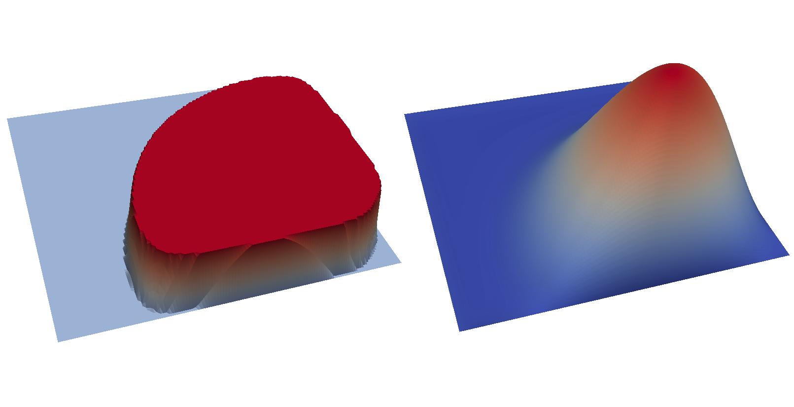
The optimal control and state can be visualised by opening
output/u.pvd and output/y.pvd in paraview. The optimal control
should look like the image on the left and the optimal state like the
image on the right:
References
| [5E-BRB08] | B.T. Baumrucker, J.G. Renfro, and L.T. Biegler. MPEC problem formulations and solution strategies with chemical engineering applications. Computers & Chemical Engineering, 32(12):2903 – 2913, 2008. doi:http://dx.doi.org/10.1016/j.compchemeng.2008.02.010. |
| [5E-HintermullerK11] | (1, 2, 3) M. Hintermüller and I. Kopacka. A smooth penalty approach and a nonlinear multigrid algorithm for elliptic MPECs. Computational Optimization and Applications, 50(1):111–145, 2011. URL: http://dx.doi.org/10.1007/s10589-009-9307-9, doi:10.1007/s10589-009-9307-9. |
| [5E-KS00] | D. Kinderlehrer and G. Stampacchia. An introduction to variational inequalities and their applications. Volume 31 of Classics in Applied Mathematics. SIAM, 2000. |
| [5E-LH04] | S. Lawphongpanich and D.W. Hearn. An MPEC approach to second-best toll pricing. Mathematical Programming, 101(1):33–55, 2004. doi:10.1007/s10107-004-0536-5. |
| [5E-LM05] | S. Leyffer and T. Munson. Solving multi-leader-follower games. Preprint ANL/MCS-P1243-0405, 4:04, 2005. |
| [5E-YG05] | K. Yunt and C. Glocker. Time-optimal trajectories of a differential-drive robot. In Proceedings of the Fifth Euromech Nonlinear Dynamics Conference, 1589–1596. 2005. |
| [5E-ZQJSD96] | Luo Z.-Q., Pang J.-S., and Ralph D. Mathematical programs with equilibrium constraints. Cambridge University Press, 1996. |
| [5E-ZBLN97] | C. Zhu, R. H. Byrd, P. Lu, and J. Nocedal. Algorithm 778: L-BFGS-B: Fortran subroutines for large-scale bound-constrained optimization. ACM Transactions on Mathematical Software, 23(4):550–560, 1997. doi:10.1145/279232.279236. |